Reading Time: 13 minutes

Formal models confirm that the intensity of political terms increases during the election period, but also show that the two rhetorical frames follow different dynamics.

1. From descriptive findings to formal testing

In the second part of the series, we saw a clear descriptive picture. The “Vučić AND Stability” frame had a higher total number of mentions and appeared in more articles. The “Blockaders AND Chaos” frame was less frequent overall, but more explosive, especially on election day. Both frames intensified after the official election announcement, but they did not follow the same temporal pattern.

Descriptive statistics are the first and necessary step. They provide an overview, but they do not answer every question. If a daily count is high, we need to ask whether this is just one unusual day or part of a more systematic pattern. If averages differ across subperiods, we need to ask whether the difference remains meaningful once the structure of the data is taken into account. If one term group has an enormous spike on election day, we need to check whether that spike dominates the whole analysis or whether there are also relevant pre-election patterns.

This is why the third part moves to models. Models are not a replacement for graphs and tables; they are their continuation. A graph shows what happened. A model helps us assess how stable that pattern is when placed in a more formal statistical framework. In this analysis, models are fitted only to the daily term-count series. Article counts and saturation are used descriptively and graphically, because saturation is not a count variable of the same type as daily mentions.

Tabel 1. Simplified table of key model results

Model	Term/window	IRR	95% CI	p-value	Interpretation
Pooled negative binomial model	Vučić vs Blokader	1.2	0.96–1.55	0.104	Vučić/Stability has a higher expected number than Blokader/Chaos, but the difference is not statistically significant at the 5% level.
Pooled negative binomial model	-30 to -15 days before the election	1.6	1.06–2.33	0.023	The expected number of occurrences is statistically higher than in the reference period outside the election windows.
Pooled negative binomial model	-14 to -8 days before the election	2.3	1.28–3.95	0.005	The expected number of occurrences is statistically higher than in the reference period outside the election windows.
Pooled negative binomial model	-7 to -1 day before the election	1.8	1.03–3.19	0.038	The expected number of occurrences is statistically higher than in the reference period outside the election windows.
Pooled negative binomial model	Election day	10.4	2.41–44.67	0.002	The total expected number of appearances is many times higher on election day.
Pooled negative binomial model	+1 to +7 days after the election	1.6	0.92–2.85	0.092	The finding is borderline/suggestive: the expected number is higher, but with lower statistical certainty.
Pooled negative binomial model	+15 to +30 days after the election	1.5	0.99–2.16	0.059	The finding is borderline/suggestive: the expected number is higher, but with lower statistical certainty.
Interaction negative binomial model	Vučić × -30 to -15	2.3	1.07–5.02	0.034	Vučić/Stability is relatively more pronounced than Blokader/Chaos in the earlier pre-election window.
Interaction negative binomial model	Vučić × election day	0.2	0.01–3.34	0.261	The direction shows that the electoral jump is relatively weaker for Vučić/Stability than for Blokader/Chaos; in the NB model the interval is wide.
Term-specific negative binomial model: Blokader	Election day	18.1	2.17–150.37	0.007	For Blokader/Chaos the main robust finding is an extremely large selection jump.
Term-specific negative binomial model: Vučić	Election day	3.0	0.45–20.30	0.258	There is not strong enough model evidence for the particular effect of this window.
Term-specific negative binomial model: Vučić	-30 to -15 days before the election	2.5	1.47–4.09	<0.001	For Vučić/Stabilost, this pre-election window is statistically higher compared to the reference period.
Term-specific negative binomial model: Vučić	-14 to -8 days before the election	3.3	1.59–6.89	0.001	For Vučić/Stabilost, this pre-election window is statistically higher compared to the reference period.
Term-specific negative binomial model: Vučić	-7 to -1 day before the election	2.1	1.01–4.38	0.048	For Vučić/Stabilost, this pre-election window is statistically higher compared to the reference period.
Term-specific negative binomial model: Vučić	+1 to +7 days after the election	2.2	1.04–4.53	0.039	For Vučić/Stabilost, the first post-election window remains statistically elevated.

In these posts, only the main results are given in summary form. All analysis outputs are provided in a zip file containing all graphics (png format) and tables (in Word, Excel and CSV format).

output_count_pair_analysis_kurirDownload

Intuitively, this third part answers the question: does what we saw in the descriptive tables remain visible when we use models designed for count data? The answer is broadly yes, but with important nuances. The models confirm that term intensity increases during the election period, especially around election day. At the same time, they show that “Blockaders AND Chaos” and “Vučić AND Stability” do not intensify in the same way.

2. Why ordinary linear regression is not used

The first methodological step is to understand the nature of the dependent variable. In this analysis, we are not measuring temperature, an index, a percentage, or a score on a scale. We are measuring how many times a group of terms appeared in a day. These are count data: 0, 1, 2, 3, and so on. They cannot be negative, they are often asymmetric, and they may contain large spikes.

Ordinary linear regression is not ideal for such data. It can predict negative values, even though a negative number of term mentions has no meaning. It also assumes a different error structure from the one usually found in count data. In daily media counts, we often see quieter periods, sudden spikes, and then a return to lower levels. This dynamic is much closer to count models than to standard linear regression.

For that reason, we use models for count data. Their basic idea is simple: rather than estimating an ordinary continuous outcome, the model estimates the expected number of events. In this case, the event is a term mention on a given day. The model asks: how many mentions should we expect for a given frame, in a given election window, taking the day of the week into account?

This is important for non-specialist readers. The model does not “read” the articles and does not understand political intent. It only links daily counts to time markers: before the election, immediately before the election, election day, after the election, and so on. In this way, the descriptive pattern is translated into a statistically testable form.

Count data are non-negative integers. This is why Poisson, quasi-Poisson, and negative binomial models are more appropriate than ordinary linear regression.

In short, models are needed because the number of word mentions is not an ordinary continuous variable. If we want to analyse daily term counts seriously, we need a tool that respects their count-data nature.

3. The Poisson model: a useful starting point, but not the final word

The best-known model for count data is the Poisson model. Intuitively, the Poisson model is used when we count how many times an event occurred in a given interval: the number of calls, accidents, posts, or term mentions. In this analysis, the event is the appearance of a given group of terms on a given day.

The Poisson model has a simple logic. It estimates the expected daily count as a function of explanatory factors. These factors can include which term group is being analysed, which election window is involved, and which day of the week it is. For example, the model can compare the expected number of mentions in the final seven days before the election with the period outside the election windows.

However, the Poisson model has one important assumption: the variance of the count data is approximately equal to their mean. In real media data, this assumption is often violated. Daily counts may be much more variable than the Poisson model expects (test statistic = 7.14, and p-value < .01). One day may have 20 mentions, another 30, another 500. Such spikes mean that variability is much larger than the average level.

This is exactly what happens in our analysis. A formal overdispersion test shows that the variability is significantly larger than a simple Poisson model would assume. For this reason, the Poisson model is used as a starting point, but not as the main model for interpreting the results.

Intuitively, the Poisson model is like a first draft of a map. It shows the basic directions, but if the terrain is much rougher than the model assumes, the map becomes too smooth. We therefore need a model that allows for more roughness, or greater variability, in the data.

4. Overdispersion: when the data are “more restless” than Poisson expects

Overdispersion means that count data are more variable than expected under the Poisson model. If the average daily count is 40, the Poisson model expects the variance to be roughly 40 as well. But if the actual daily counts are much more spread out, with large spikes and drops, the variance can be several times larger.

Why does this matter? If we ignore overdispersion, the model may appear more certain than it really is. Standard errors may be too small, p-values too optimistic, and conclusions too confident. In other words, a simple Poisson model may say that something is statistically significant partly because it failed to account for how variable the data really are.

In our results, the overdispersion test is highly significant. This means that the Poisson model is too restrictive for these data. Daily counts of terms in the Politics section of Kurir.rs are not calm and even. They contain periods of lower intensity, periods of higher intensity, and very large spikes, especially for the “Blockaders AND Chaos” frame on election day.

For this reason, the main interpretation should rely on the negative binomial model and, as a supplementary check, the quasi-Poisson model. These models are more flexible because they allow greater variability than the ordinary Poisson model.

“What is overdispersion?” — The most important intuitive meaning of overdispersion in this analysis is this: the data are too explosive for a simple model that expects relatively calm count values. Moving to the negative binomial model is therefore not a technical detail, but a key methodological step.

When the daily numbers are much more variable than the Poisson model expects, we use more flexible models such as the negative binomial or quasi-Poisson model.

5. The negative binomial model: a more flexible model for explosive count data

The negative binomial model is close to the Poisson model, but more flexible. Its main advantage is that it allows the variance to be larger than the mean. This makes it especially useful for data with sudden spikes, uneven intensity, and periods of much higher activity.

In this analysis, the negative binomial model fits the data much better than the Poisson model. This is visible in the model-fit statistics. The Poisson model has an AIC of about 9475, while the negative binomial model has an AIC of about 2674. A lower AIC indicates a better balance between model fit and model complexity. The difference is very large, confirming that the negative binomial model is more appropriate for these data.

AIC (Akaike Information Criterion) is a criterion used to compare two models. It has two components, the first of which measures the degree of adaptation of the model to the data, and the second which is a measure of the complexity of the model (simplified, how many coefficients we have included in the model we are evaluating). According to the AIC criterion, a model that has a better degree of adaptation to the data (e.g. lower variance) and is simpler at the same time (has a smaller number of evaluated coefficients) is preferable.

The model includes several important factors. First, it distinguishes between the two term frames: “Blockaders AND Chaos” and “Vučić AND Stability”. Second, it includes election windows, such as 30 to 15 days before the election, 14 to 8 days before the election, the final week before the election, election day, and post-election windows. Third, it includes the day of the week, because media activity may differ between weekdays and weekends.

The negative binomial results show that the overall intensity of term mentions is significantly higher in several election windows. The election-day effect is particularly strong. In the pooled negative binomial model, election day has an incidence rate ratio of 10.38. This means that the expected daily count on election day was more than ten times higher than in the reference period, holding the other model terms constant. The reference period in our case is the period before the official election announcement, i.e. from January 1 to February 23, 2026.

This does not mean that election day “caused” every individual term mention. It means that, statistically, election day was associated with a much higher expected number of mentions in the analysed series.

6. How to read incidence rate ratios

Count-model results are often presented as incidence rate ratios, or IRRs. The term may sound technical, but the idea is quite simple. An IRR shows how much the expected count changes relative to a reference category.

If the IRR is 1, there is no difference in the expected count. If the IRR is greater than 1, the expected count is higher. If the IRR is below 1, the expected count is lower. For example, an IRR of 1.50 means that the expected count is 50% higher than in the reference period. An IRR of 2 means the expected count is twice as high. An IRR of 10 means the expected count is ten times higher.

Table 2. Pooled negative binomial models

Model	Term	Estimate	95% low	95% high	Std error	Statistic	p-value
Pooled negative binomial model	event window minus 30 to minus 15	1.57	1.06	2.33	0.20	2.27	0.023
Pooled negative binomial model	event window minus 14 to minus 8	2.25	1.28	3.95	0.29	2.83	0.005
Pooled negative binomial model	event window minus 7 to minus 1	1.82	1.03	3.19	0.29	2.08	0.038
Pooled negative binomial model	event window election day	10.38	2.41	44.67	0.74	3.14	0.002
Pooled negative binomial model	event window plus 1 to plus 7	1.62	0.92	2.85	0.29	1.68	0.092

In this analysis, several IRRs are especially important. In the pooled negative binomial model, election day has an IRR of 10.38. The period from 14 to 8 days before the election has an IRR of 2.25, and the final week before the election has an IRR of 1.82. This means that these periods are associated with higher expected daily term counts than the period outside the defined election windows.

What the IRR does not tell us is why the increase occurred. It is a measure of statistical association within the model. It does not prove intent, coordination, or effects on voters. But it helps us quantify how different a period was from the reference level.

This is why IRRs are useful for public communication. Instead of simply saying “there were more mentions”, we can say: “the model estimates that the expected number of mentions in this period was roughly two times, three times, or ten times higher than in the reference period.” That is more intuitive and more informative.

7. What the models show for “Blockaders AND Chaos”

When “Blockaders AND Chaos” is analysed separately, the strongest and most stable model-based finding concerns election day. In the term-specific negative binomial model, election day has an IRR of 18.07 and a p-value of .007. This means that the expected count for this frame on election day was about 18 times higher than in the reference period.

This finding is consistent with the descriptive picture from the second part of the series. There, we saw that election day had 521 mentions of “Blockaders AND Chaos” in 48 articles. The model now shows that this spike is not only visually impressive, but also statistically strong, even when we use a more flexible model that accounts for high variability in the data.

At the same time, the other pre-election windows for this frame are not equally stable in the term-specific negative binomial model. Descriptively, there are elevated values before the election, but once the model accounts for overdispersion and weekday effects, the strongest result remains election day.

Table 3. Term-specific models for “Blockaderi AND Chaos” and for “Vučić AND Stability”

Model	Term	Estimate	95% low	95% high	Std error	Statistic	p-value
Term-specific negative binomial model: Blokader	event window election day	18.07	2.17	150.37	1.08	2.68	0.007
Term-specific negative binomial model: Vučić	event window minus 30 to minus 15	2.45	1.47	4.09	0.26	3.44	0.001
Term-specific negative binomial model: Vučić	event window minus 14 to minus 8	3.31	1.59	6.89	0.37	3.20	0.001
Term-specific negative binomial model: Vučić	event window minus 7 to minus 1	2.10	1.01	4.38	0.38	1.98	0.048
Term-specific negative binomial model: Vučić	event windowplus 1 to plus 7	2.17	1.04	4.53	0.38	2.07	0.039

Intuitively, this means that the “Blockaders AND Chaos” frame is explosive in character. It is not merely slightly elevated throughout the campaign; it culminates at the most politically sensitive moment. This does not prove why it happened, but it clearly shows when it happened and how strong the spike was relative to the usual level.

8. What the models show for “Vučić AND Stability”

For the “Vučić AND Stability” frame, the model shows a different dynamic. Instead of one dominant election-day spike, this frame is systematically elevated across the broader pre-election period.

In the term-specific negative binomial model, the period from 30 to 15 days before the election has an IRR of 2.45 and a p-value of .0006. The period from 14 to 8 days before the election has an IRR of 3.31 and a p-value of .0014. The final week before the election has an IRR of 2.10 and a p-value of .0476. The first week after the election is also elevated, with an IRR of 2.17 and a p-value of .0386.

These results are clear. The “Vučić AND Stability” frame is not primarily tied to one extreme election-day spike. It is elevated across several pre-election windows and remains elevated immediately after the election. This supports the interpretation from the second part of the series: stability functions as a broader, more durable, and more persistent campaign frame.

Intuitively, this model says that the stability frame behaves differently from the chaos frame. Stability is not only a reaction to election day. It is built across the pre-election period, appears in several campaign phases, and remains visible immediately after election day. This model-based result fits well with the descriptive picture of broader and more continuous presence.

9. Interactions: do the two frames intensify in the same way?

Interaction models ask an additional question: do “Vučić AND Stability” and “Blockaders AND Chaos” change in the same way across the same election windows? In other words, we are not asking only whether the terms intensify, but whether one frame intensifies more or earlier than the other.

The most important interaction result shows that “Vučić AND Stability” is relatively stronger than “Blockaders AND Chaos” in the earlier pre-election window, from 30 to 15 days before the election. The interaction negative binomial model gives an IRR of 2.31 for this difference, with a p-value of 0.034. This suggests that the stability frame was especially pronounced in the earlier stage of the pre-election period.

On the other hand, election day is relatively much stronger for “Blockaders AND Chaos”. The interaction models point in that direction, although the level of statistical certainty differs across model types. Substantively, this is consistent with the descriptive evidence: election day is dramatic for the chaos frame, while stability is more widely distributed across the pre-election period.

Table 4. Interaction results

Model	Term	Estimate	95% low	95% high	Std error	Statistic	p-value
Interaction negative binomial model	term display Vučić: event window minus 30 to minus 15	2.31	1.07	5.02	0.40	2.12	0.034
Interaction negative binomial model	term display Vučić: event window election day	0.20	0.01	3.34	1.44	-1.12	0.261
Interaction quasi-Poisson model	term display Vučić: event window minus 30 to minus 15	2.34	1.19	4.62	0.35	2.45	0.015
Interaction quasi-Poisson model	term display Vučić: event window election day	0.20	0.06	0.66	0.61	-2.65	0.009

This section is important because it prevents an overly simple interpretation. It is not enough to say that both frames intensified. We need to say how they intensified. The models suggest that the stability frame intensified earlier and more broadly before the election, while the chaos frame was especially concentrated on election day. This is the key difference between the two forms of political framing.

10. Change-points: when the statistical behaviour of the series changes

In addition to regression models, the analysis uses change-point detection. Change-points are dates around which the statistical behaviour of a series changes. This may involve a change in the average level, variability, or both. It is important to emphasise that a change-point does not explain the cause of a change. It only marks that the series behaves differently around that date.

The results are interesting. For the total term count, change-points are detected around 28 March and 1 April, immediately around election day. For “Blockaders AND Chaos”, change-points appear around 28 and 30 March, consistent with the enormous election-day spike. For “Vučić AND Stability”, change-points appear around 21 and 24 February, around the period of the official election announcement.

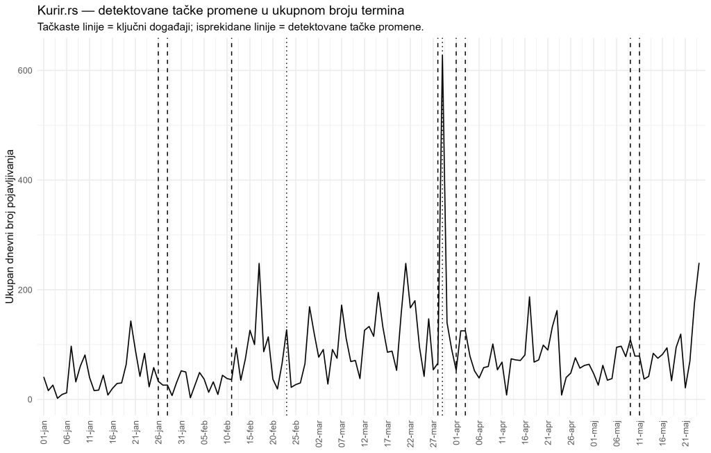
Table 5. Detected change-points in the total term counts

Change point index	Date	Total term count	Days to announcement	Days to election
26	26/01/26	33	-28	-62
28	28/01/26	26	-26	-60
42	11/02/26	36	-12	-46
87	28/03/26	66	33	-1
91	1/04/26	53	37	3
93	3/04/26	125	39	5
129	9/05/26	109	75	41
131	11/05/26	79	77	43

Table 6. Detected change-points for each term

Term display	Change point index	Date	Days to announcement	Days to election
Blokader	38	7/02/26	-16	-50
Blokader	40	9/02/26	-14	-48
Blokader	42	11/02/26	-12	-46
Blokader	44	13/02/26	-10	-44
Blokader	87	28/03/26	33	-1
Blokader	89	30/03/26	35	1
Blokader	131	11/05/26	77	43
Blokader	133	13/05/26	79	45
Vučić	37	6/02/26	-17	-51
Vučić	39	8/02/26	-15	-49
Vučić	52	21/02/26	-2	-36
Vučić	55	24/02/26	1	-33
Vučić	111	21/04/26	57	23
Vučić	113	23/04/26	59	25

These results support the main interpretation of the series. The stability frame changes around the entry into the election period, while the chaos frame changes dramatically around election day itself. Still, change-point results should be used as supporting evidence, not as the sole basis for a conclusion. Algorithms can also detect short local bursts, so every important date should be checked through qualitative reading of the articles.

11. What the models confirm, and what they cannot prove

The models confirm several important points. First, the data are too variable for a simple Poisson model, so the negative binomial model is more appropriate. Second, overall term intensity is elevated during the election period, especially on election day. Third, “Blockaders AND Chaos” has a strong and statistically robust election-day spike. Fourth, “Vučić AND Stability” is systematically elevated across the broader pre-election period and immediately after the election. Fifth, the two frames have different dynamics, not just different total numbers of mentions.

But the models do not prove intent. They cannot show that someone ordered the use of particular expressions. They cannot prove coordination. They cannot show effects on voters. They cannot demonstrate that every article had the same political function. They model daily term counts and their association with time windows.

That is enough for a serious finding, but not enough for exaggerated claims. The most precise formulation would be: the data show a systematic increase in the analysed rhetorical frames during the election period, with different dynamics across the two frames. The stability frame has a broader pre-election character, while the chaos frame culminates on election day.

This is a methodologically important conclusion. It shows how media language can be analysed in a disciplined way: first descriptively, then through models, and finally with a clear distinction between what statistics can show and what they cannot prove.

12. Short technical appendix

The Poisson model is a standard model for count data. It is used when we count how many times an event occurred in a given interval. In this analysis, the event is the appearance of a group of terms on a given day. The Poisson model is useful as a starting point, but its assumption that the mean and variance are approximately equal is often unrealistic for media data.

Overdispersion occurs when the variance is larger than the mean. In such cases, the Poisson model may underestimate uncertainty. More flexible models, such as the quasi-Poisson and negative binomial models, are therefore used. The negative binomial model is especially useful when count data are explosive, with large spikes and uneven variability.

An incidence rate ratio shows how much the expected number of events is higher or lower relative to the reference category. An IRR of 2 means that the expected count is twice as high. An IRR of 0.5 means that the expected count is half as high.

Useful references for readers who want more technical detail include Gardner, Mulvey, and Shaw on the problems of linear regression and Poisson models for overdispersed count data, and Zeileis, Kleiber, and Jackman on count models in R. The latter paper explains classical Poisson, geometric, and negative binomial regression models for count data and their implementation in R.

References for the technical appendix

Gardner, W., Mulvey, E. P., & Shaw, E. C. (1995). Regression analyses of counts and rates: Poisson, overdispersed Poisson, and negative binomial models. Psychological Bulletin, 118(3), 392–404. https://doi.org/10.1037/0033-2909.118.3.392

Zeileis, A., Kleiber, C., & Jackman, S. (2008). Regression models for count data in R. Journal of Statistical Software, 27(8), 1–25. https://doi.org/10.18637/jss.v027.i08

The conclusion of this third part is that formal models do not replace descriptive analysis; they discipline it. They confirm that the election period is not only visually different, but statistically associated with higher expected counts of politically meaningful terms. At the same time, the models show that the two frames do not have the same temporal function: stability is built across the campaign period, while chaos culminates on election day.