Reading Time: 7 minutes

Part I asked which kinds of data belong in an election forecast. The second problem is less glamorous but often more important: when were those data actually known?

At first this sounds like data administration. In practice, it can determine whether we have reconstructed a genuine historical forecast or performed a sophisticated trick in which a 2022 model quietly receives information published in 2023 and is then praised for its remarkable foresight. Chapter 3 therefore argues that election forecasting requires not merely good data but a reconstruction of the information set that genuinely existed at the forecast date.

The best predictor of an election is a result that was not yet known

Imagine testing how well our model would have forecast an earlier Serbian election. Today we download the latest statistical series on employment and wages, use current demographic estimates, add final official election results and a modern classification of party coalitions, and obtain a spectacular historical fit.

The difficulty is that today’s historical database is not necessarily the database a real forecaster could have used before that election. Economic statistics may have been revised. Demographic estimates may incorporate information that arrived later. Coalitions that now look obvious may not yet have existed. Even a poll included in the database may have completed its fieldwork after the date on which our supposedly historical forecast was frozen.

The model has not necessarily discovered a deep political law. It may simply have seen the future through the back door. This is look-ahead bias, and it can produce exactly the kind of beautiful retrospective chart that makes analysts begin to believe they have discovered political physics.

Different data live on different clocks

A forecasting database also contains variables that operate on very different schedules. Polls arrive irregularly. Inflation and employment are usually monthly. GDP is quarterly. Census data appear occasionally. Media and digital indicators may be daily or nearly continuous. Election results, fortunately for voters and inconveniently for statisticians, occur only once per electoral cycle.

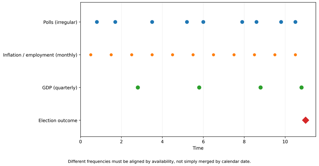
Figure 3.2. Data at different temporal frequencies. Polls, monthly indicators, quarterly GDP and election outcomes do not become available simultaneously merely because they can be placed on the same calendar.

Simply joining everything by date creates the illusion that all information was known at the same time. If first-quarter GDP is released in May, a forecast made on 15 April cannot use it merely because the statistic refers to January–March. The reference period answers what the observation describes. The release date answers the more important forecasting question: when could the analyst actually have known it?

A statistic can describe the past and still belong to the future

This is one of the most important and least glamorous ideas in the book. Every observation has at least two clocks: the period it describes and the date it first became available. Revised statistics create a third. The forecast itself then has a cutoff — the precise moment after which no new information is allowed to enter that version of the forecast.

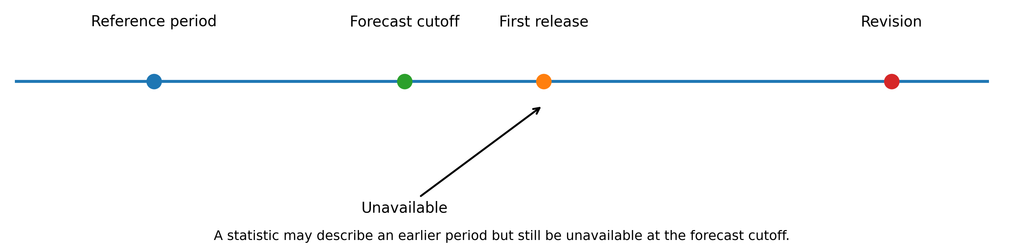
Figure 3.3. The data-release problem. A statistic may describe an earlier period, but if it was first released after the forecast cutoff, the historical forecaster could not have known it.

This matters enormously in retrospective evaluation. Today’s historical economic series are often cleaner than the data available in real time. If we give the model the revised past and then admire its performance, we have organised a competition in which one contestant received the answers before the exam.

Ipsos before polls closed and Ipsos after polls closed were solving different problems

Serbia’s 25 October election provides an unusually clear illustration. Three days before voting, Ipsos estimated United Serbia at 47.4%, the Student List at 40%, and turnout at 64.7%. As discussed in Part I, the research had a clearly described sample, data-collection method and commissioner.

After the polling stations closed, CeSID and Ipsos were no longer relying primarily on respondents telling them what they intended to do. They used a stratified sample of 750 actual polling stations and collected election-day turnout and result data. Their final projection on 100% of the sample put the Student List at 53.0% and 141 seats and United Serbia at 38.8% and 103 seats, very close to the preliminary official results.

This is not a story in which “Ipsos forgot statistics on Thursday and remembered them on Sunday”. These are fundamentally different information problems. Before the election, we measure preferences and predict behaviour that has not yet occurred. After polls close, we sample an outcome that has already happened. The second type of information is much closer to the target.

CRTA used the same logic with its random representative sample of 500 polling stations and estimated the Student List at 52.45% and United Serbia at 39.2%. This is why a serious database should distinguish a pre-election survey, a pre-election forecast, an election-night sample projection, and the official result. They are all “election data”, but they are not the same data product.

Thousands of polling stations are not thousands of elections

A second illusion appears when we move from the national level to municipalities and polling stations. Serbia has thousands of polling stations, so the database suddenly looks enormous. That is extremely useful for geographical analysis, turnout modelling, local patterns and election forensics. But several thousand rows do not mean several thousand independent parliamentary elections.

All those polling stations share the same election day, electoral law, much of the national campaign, and many common political shocks. “I have 8,000 polling stations” is therefore statistically very different from “I have 8,000 independent elections”. Chapter 3 explicitly warns against confusing the number of database rows with the amount of independent historical information.

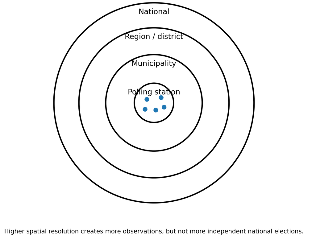
Figure 3.4. Geographic resolution of a Serbian election-forecasting database. Finer spatial resolution gives more detailed observations, but it does not create additional independent national election cycles.

This is also where the ecological fallacy enters. If municipalities with more public-sector employment also give more votes to the government, we cannot infer automatically that public-sector employees themselves produced the higher government vote. Age structure, settlement type, education, local economic conditions, or other factors may explain the municipal pattern. A municipal correlation is not individual behaviour.

Parties have the inconvenient habit of changing their names, partners and relatives

Political lists create another difficulty for historical data. Parties split, merge, enter new coalitions, create new lists, and sometimes preserve an old label while changing much of the organisation behind it. If A and B contest one election together, but next time A joins C while B competes alone, what exactly is the “previous vote” for A+C?

There is no purely technical answer. It is a modelling decision. Chapter 3 therefore separates the legal identity of a party, the official identity of an electoral list, and the analytical lineage used by the researcher.

This is particularly relevant in Serbia, where coalition structures can change faster than analysts can rename spreadsheet columns. If historical votes are transferred from one configuration to another, that decision should be documented. It should not disappear under the harmless-looking heading “data cleaning”, because an analytical assumption has just been made.

Missing is not always the same kind of missing

Another apparently small issue becomes important later: not every empty cell means the same thing. A value may never have been measured. It may exist but have remained unpublished. It may be scheduled for publication but not yet have been available at the forecast date. Or it may be conceptually inapplicable, as when a completely new electoral list has no previous result.

Coding all of these as one generic NA discards information. The first case is a measurement problem, the second a transparency problem, the third a real-time availability problem, and the fourth a feature of the political structure itself. A good forecasting system records not only that a number is missing, but why.

Reproducibility means more than “the code is on GitHub”

Publishing code is excellent, but it is not enough. Run the same script next year using a revised historical economic database and the reconstructed “historical forecast” may change. Chapter 3 therefore calls for a traceable chain from the published forecast backwards: model run, model version, processed dataset, historical raw-data vintage, and original source.

Every public forecast should preserve its cutoff date, code version, data versions, party-lineage mapping, and important model settings. If simulation is used, saving the simulation draws is valuable as well. None of this is particularly exciting television material, but it allows a serious answer years later when someone asks: “What exactly did you know when you published this?”

So who was “most accurate”?

The predictable post-election competition has already begun. Vreme reviewed several public pre-election estimates and concluded that BIRODI’s central scenario was numerically closest to the realised result, while Ipsos and Faktor Plus had even selected the wrong winner. NSPM had the correct ordering of the leading lists but anticipated a much smaller gap than the one observed.

That comparison is informative, but professional evaluation requires us to define what “most accurate” means before seeing the result. Are we measuring mean absolute error across all lists? Only the two largest? Turnout? Threshold classification? Seats? Are we comparing a survey fielded several months earlier with an estimate produced three days before voting? Do we include an analytical model that explicitly described itself as a scenario rather than a conventional poll?

If we choose the metric after the election, almost every forecasting organisation can find a category in which it won. Here we return to the same principle that governs data selection: the rules should be specified before we see the answer.

BIRODI’s relatively good result is therefore a reason to examine its model seriously. It is not a reason to canonise it after one election cycle. Likewise, Ipsos’s large pre-election miss does not demonstrate that every survey the organisation has ever conducted is worthless. The more useful question is which component failed, preference measurement, turnout modelling, undecided-voter treatment, common polling error, or some other part of the process.

The database is part of the model

Chapter 3 ultimately proposes that a Serbian election-forecasting system should not be one giant spreadsheet but a connected research infrastructure: elections, electoral lists, party lineage, polls, polling-station results, demographics, economics, media, regime-sensitive indicators, digital traces, forensic flags, data vintages, and every individual forecast run.

This may sound less exciting than asking who will win next Sunday, but it determines whether we will later be able to tell the difference between a genuinely good forecasting system and a model that was merely lucky.

The most important question for a new variable is therefore not: “Can we download it?”

A better question is: What does it measure, when could we have known it, where does it belong, and does it actually improve the forecast?

If we cannot answer those questions, perhaps we do not need more data. Perhaps we need better discipline.