Reading Time: 7 minutes

This post continues my series on election forecasting, based on a book I am currently preparing. The purpose remains the same: to put some of the book’s ideas into the public domain before the manuscript is final, in language useful both to specialists and to readers who do not spend their spare time studying sampling frames and predictive distributions. If criticism shows that something is unclear, overstated, or unnecessarily technical, that is useful information while the book can still be improved.

The previous posts focused on what a poll actually measures and why the same percentage need not mean the same thing in different political environments. This time I want to step back from a single poll and look at the entire warehouse of information available to a modern election forecaster. The old problem of data scarcity has increasingly been replaced by a new one: we can collect almost everything, but we still have to decide what any of it is for. Chapter 3 starts from precisely this warning: more data can produce a worse forecast rather than a better one.

When a spreadsheet with 200 columns starts to look like science

Polls, previous election results, inflation, wages, employment, age, education, local demographics, government approval, television exposure, media tone, protests, Google searches, Facebook, X, TikTok, likes, shares, and probably something invented before I finish the book can all be turned into variables.

That creates a seductive intuition. If one model has ten variables and another has one hundred, the second must know more. Not necessarily. Search through enough variables after seeing the outcome and some will fit previous elections spectacularly well by chance. A model built around those discoveries may look brilliant in retrospect and collapse at the next election. Chapter 3 therefore imposes a simple discipline: every variable should have an analytical role before it earns a place in the forecasting database.

A poll is not inflation, and Google is not a voter

For practical purposes, election-forecasting data can be divided into four broad families. The first contains direct electoral measurements: polls, previous results, turnout, votes, and polling-station information. The second contains structural information and electorate composition: demographics, employment, income, education, geography, and similar variables that may inform turnout models or structural expectations.

The third family describes political context: media exposure, protest activity, public-sector dependence, indicators of political pressure, administrative mobilisation, or pre-defined election-integrity measures. The fourth consists of experimental and digital signals, Google Trends, social-media activity, sentiment measures, and other fast and fashionable data streams. Trouble begins when we treat all four families as if they were simply different thermometers measuring the same political temperature. They are not.

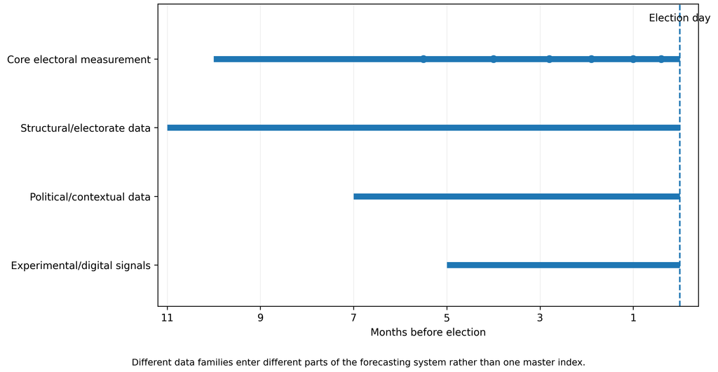
Figure 3.1. One election forecast, four layers of data. Different data families can contribute to the same forecasting system, but they do not measure the same phenomenon and should not be mechanically combined into one electoral index.

A good model therefore asks more than whether a variable correlates with election results. It asks what the variable measures. A poll attempts to measure reported political preference. Demographics describe the population to which we want to generalise. Inflation may contribute to a structural expectation about an incumbent government, but inflation is not a hidden poll. Media exposure measures an information environment, but fifteen minutes of television coverage is not fifteen additional votes. A Google search for a politician indicates attention, but attention may mean support, anger, scandal, or simply curiosity about the latest extraordinary statement.

Ipsos three days before the election: why metadata matter

Serbia’s October election provided an almost textbook illustration. On 22 October, Ipsos published an estimate based on research conducted from 20 to 22 October with 3,624 respondents. It projected Aleksandar Vučić – United Serbia at 47.4%, the Student List at 40%, and Ivica Dačić’s list at 3.2%, with expected turnout of 64.7%. The commissioner was the Aleksandar Vučić – United Serbia electoral list. Ipsos also disclosed important methodological information: target population, mixed telephone/online collection, treatment of decided voters, and an assumption of 2.5% invalid ballots.

A political list commissioning a poll does not automatically invalidate it. It does, however, make transparent metadata and a strong professional boundary between the client’s interests and the analytical procedure particularly important. A professional polling organisation should not alter methods, interpretations, or presentation because of who pays for the research. If a result is released publicly as an analytical product, readers should be able to see how it was produced, what assumptions were added, and which forms of uncertainty are not captured by the usual sampling margin.

The preliminary results established by Serbia’s Republic Electoral Commission on 26 October at 20:00, based on 97.56% of processed polling stations, put the Student List at 52.71%, United Serbia at 39.17%, and Dačić’s list at 2.17%. Those figures are very far from the pre-election Ipsos estimate, and both leading-list results were well outside the intervals Ipsos had published alongside its estimates.

That does not make every statistical interval “wrong”. It demonstrates that an interval driven primarily by sampling uncertainty does not automatically capture total forecast uncertainty: non-response, turnout misspecification, coverage problems, correlated polling error, late mobilisation, or genuine last-minute movement may all matter. Once a survey estimate is presented as an estimate of the final election result, the analytical burden becomes greater, not smaller.

The same data, a different headline

The media framing is also instructive. Alo described the Ipsos result in its headline as United Serbia being “convincingly in first place with 47.4 percent”. The article itself reproduced substantial methodology, including the commissioner, but the headline had already given the reader a political frame through which to interpret the numbers.

Politika used the more descriptive “Vučić’s list at 47.4 percent, Student List at 40 percent”, while Danas explicitly reported the commissioner, the use of decided voters as the denominator, the mixed survey mode, and the additional invalid-ballot assumption.

This is a useful reminder that even when the same numbers are reproduced accurately, the headline is part of the interpretation. Pollsters cannot control every headline, but they can make political repackaging harder by distinguishing clearly between what was observed, what was assumed, what was modelled, and what remains uncertain.

CRTA, NSPM, and Faktor Plus are not three interchangeable spreadsheet rows

As discussed in the previous post, the recent Serbian surveys differed substantially. CRTA’s June face-to-face survey of 2,324 adults put the Student List at 44.9% and SNS at 35.7% among decided respondents. NSPM’s telephone survey conducted from 25 September to 5 October with 1,050 respondents put the Student List at 44.5% and United Serbia at 42.7% among declared respondents. Faktor Plus, using research from 16 to 20 September with 986 respondents, reported United Serbia at 48.6% and the Student List at 37.1%.

The least useful thing we can do is put those percentages into adjacent columns and behave as if they differ only because one pollster is “better” or “worse”. They were conducted at different times, using different modes, with different ways of handling undecided respondents and potentially different target populations. This is why the Chapter 3 polling database stores not just a percentage but also pollster, commissioner, fieldwork start and end, publication date, sample size, target population, survey mode, weighting information, treatment of undecideds, original source, download date, and subsequent corrections.

In other words, 44.5 is not complete information. Without metadata, it is simply a number waiting for a political owner.

Demography matters, but it is not another poll

Demographic data have a different job. Age, education, region, urbanisation, and employment help us understand who constitutes the electorate and whether a survey sample resembles the population to which we want to generalise. Later chapters use these data for turnout modelling and MRP, but the important point here is conceptual: demographic structure is not another approval rating.

The same confusion occurs with economic information. Inflation, real wages, unemployment, or government approval may contain predictive information, but they should not be thrown into a poll average as though they were additional respondents. Serbia also faces a particular limitation: the number of genuinely independent national parliamentary elections relevant to a modern model is small. We may have hundreds of monthly economic observations, but we do not have hundreds of independent Serbian elections. More rows do not automatically create more history.

“Clientelist municipality” is not a variable

Political context is even more delicate. If public-sector dependence may influence mobilisation, it is better to measure the share of public-sector employment than to label a municipality “clientelist”. If media inequality matters, we should measure exposure, airtime, tone, reach, or visibility rather than entering “unfair media” as a subjective score. Chapter 3 asks us to turn politically suggestive labels into measurable hypotheses.

BIRODI, for example, published monitoring before the election according to which United Serbia was presented almost exclusively positively on Informer TV, while the Student List was presented almost exclusively negatively. Such monitoring can be strong evidence about media imbalance and can be an important political-context variable. But even a precisely measured number of television minutes does not tell us automatically how many percentage points of vote share it produced. Those are different questions, and a serious data architecture should keep them different.

Google knows what we search for, not how we will vote

Digital data are particularly seductive because they are abundant and fast. If Google searches for a politician suddenly explode, it is tempting to think we have discovered an electoral wave before traditional polling has noticed it. The problem is that Google cannot tell whether the search reflects support, anger, scandal, curiosity, or a desire to understand why the internet has once again caught fire.

The same applies to social media. Ten thousand interactions are not ten thousand voters. A small number of highly active users, activists, automated accounts, journalists, and platform algorithms can create enormous activity without producing anything remotely representative of the electorate. Chapter 3 therefore keeps digital traces in the experimental layer until they demonstrate additional predictive value on elections that were not used to discover the relationship in the first place.

Where does BIRODI fit?

At the end of August, BIRODI published a model combining official election results, several polling sources, including CRTA, NSPM, Faktor Plus, Nacija TV and Ipsos, demographic change, turnout modelling, and Monte Carlo simulation. Its central scenario gave the Student List 48.5% and the SNS/Vučić list 38.6%. Importantly, BIRODI stressed that this was not a conventional poll and described it as an analytical model/scenario rather than a simple survey result.

After the election, Vreme compared several publicly available pre-election estimates and concluded that BIRODI’s model was numerically the closest, while Ipsos and Faktor Plus had predicted the wrong winner. That is interesting and deserves analysis, but one good election does not prove that every component of a complex model is useful. Serious evaluation requires repeated elections, a scoring rule specified in advance, and testing in which we do not change the rules after seeing the result.

Even when our model comes closest, methodology does not become optional.

Give every variable a job before giving it a column

The central message of this first half of Chapter 3 is therefore not “collect everything”. For every new variable, ask first what job it is supposed to perform. Does it measure support? Describe the population? Inform turnout? Create a structural prior? Measure political context? Or is it still an experimental signal that deserves testing but not production status?

Only after that comes the question of whether the variable genuinely improves forecasting.

Perhaps the simplest defence against big-data romanticism is this: before adding a new column to the model, we should know why it is there. If we do not, it is not new evidence.

It is just another column.