Reading Time: 10 minutes

Series: “Election Forecasting: Between Statistics, Politics, and Uncertainty” — Election Forensics

When a percentage looks more precise than it really is

Imagine two television programmes discussing the forthcoming parliamentary election. On the first, an analyst confidently announces that List A will receive 41% of the vote. On the second, another analyst offers exactly the same estimate. Viewers might reasonably conclude that election experts have finally agreed on something. In Serbia, that alone could qualify as news.

However, the first analyst expects the result to fall between 40% and 42%, while the second considers a range between 35% and 47% plausible. Both have the same central estimate, but they are not making the same forecast. The first expresses considerable confidence, while the second acknowledges a much wider range of possible electoral outcomes.

In the previous article, we examined why an opinion poll, a nowcast, a scenario, and an election forecast are not interchangeable concepts. We now turn to another fundamental question: even when we know what is being forecast, how confident should we be in the result?

This question is particularly important in Serbia, where public discussion of opinion polls often revolves around comparing a few percentages. In a highly polarised political environment, these numbers can quickly become arguments for inevitable victory, certain defeat, or an assured parliamentary majority. Statistical uncertainty disappears, almost as if it were an unwelcome guest deliberately excluded from the press conference.

The same percentage does not mean the same forecast

A serious election forecast should contain more than one number. Its central estimate describes where the model places the middle or typical part of the expected outcomes, depending on how that estimate is defined. However, it does not reveal how far other plausible outcomes may lie from that central value.

This is why predictive intervals matter. Suppose a model gives List A a central estimate of 41% and an 80% predictive interval ranging from 35% to 47%. Under the model's assumptions and available information, approximately 80% of its predictive distribution lies within those boundaries. The remaining 20% lies outside them.

Such an interval is not a guarantee that the eventual result will fall within its boundaries. Nor is it automatically evidence of a reliable model. Predictive intervals are meaningful only in relation to the assumptions used to construct them. A model that overlooks an important political mechanism may produce impressively narrow intervals while being seriously overconfident.

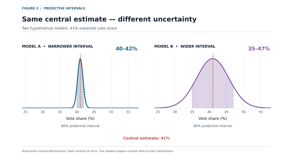
[FIGURE 3 — Two predictive distributions with an identical central estimate of 41%, but different 80% predictive intervals: 40–42% and 35–47%.]

Now imagine that List A eventually receives 45%. The second model had explicitly treated such an outcome as plausible. The first model, with its much narrower interval, had assigned considerably less probability to a result that far from its central estimate.

If we evaluated only central estimates, both models would have the same absolute error of four percentage points. Yet such an assessment would ignore an important difference in their treatment of uncertainty.

Forecast evaluation must examine not only whether the central estimate was close to the eventual result, but also whether the model expressed uncertainty appropriately.

What does a 68% probability of victory mean?

Suppose a forecasting model estimates that List A has a 68% probability of finishing first. In political reporting, this can easily become “List A is certain to win”. That headline may be convenient for a campaign, but it is not a correct interpretation of probability.

A probability of 68% means that, according to the model and its assumptions, victory is more likely than defeat. It also means that the alternative outcomes collectively retain a 32% probability.

If List A eventually loses, the forecast is not automatically wrong. An outcome that the model regarded as less likely has occurred. It would be quite different if the model had assigned List A a 99% probability of victory.

This does not mean that probabilistic forecasts are beyond criticism. Quite the opposite: they should be evaluated using repeated predictions, appropriate statistical scoring methods, and tests of calibration.

One isolated electoral outcome cannot establish whether a forecasting system consistently assigns realistic probabilities. Political commentators may prefer to award a trophy to whoever predicted the winner, but probabilistic forecasting requires more than a winners-and-losers table.

Serbia: why 3.1% can matter more than 40%

Serbia's electoral system makes the consequences of uncertainty particularly interesting. In parliamentary elections, 250 seats are allocated using the D'Hondt method. Ordinary electoral lists generally need at least 3% of the votes cast by participating voters to qualify for seat allocation. Special provisions apply to officially recognised national-minority lists.

Now imagine a hypothetical parliamentary election in which the central estimates are as follows: List A — 39%, List B — 34%, List C — 3.1%, and List D — 2.8%. Other and minority lists receive the remaining votes. For simplicity, assume that all percentages are expressed on a basis consistent with the legal electoral threshold.

At first glance, Lists A and B appear to be the principal forecasting problem because they attract the largest shares of the vote. Yet from the perspective of parliamentary composition, Lists C and D may create particularly consequential uncertainty because they are situated immediately around the threshold.

Suppose List C has a central forecast of 3.1%, but crosses the threshold in only 54% of the model's simulated election outcomes. Reporting simply that “List C is on 3.1%” may create the misleading impression that parliamentary representation is practically assured.

A more informative statement would be: “The central forecast for List C is 3.1%, but the model estimates only a 54% probability of crossing the electoral threshold.”

In other words, parliamentary representation remains highly uncertain.

List A might have a central forecast of 39% and an 80% predictive interval ranging from 36% to 42%. Although its uncertainty in percentage points is much greater, the list is comfortably above the ordinary electoral threshold in virtually every plausible outcome.

For List C, by contrast, a shift of just a few tenths of a percentage point may determine whether it participates in the allocation of seats at all. Such a result can also affect the number of seats received by other lists.

This is an example of nonlinearity: a relatively small difference in votes near an institutional threshold may create a much larger change in political representation.

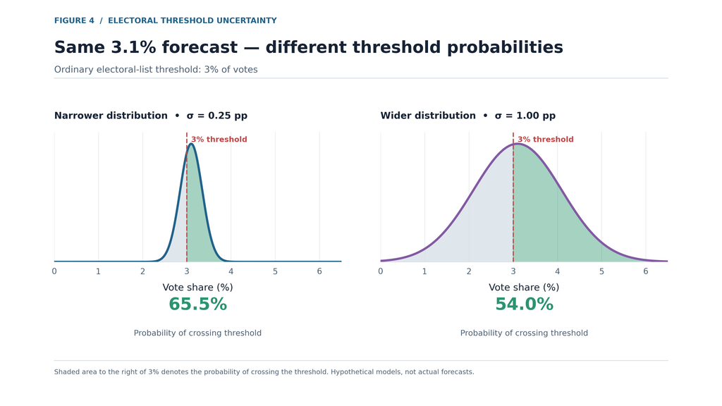
[FIGURE 4 — Two forecasting distributions centred on 3.1%, with a vertical line marking the 3% electoral threshold.]

Monte Carlo: ten thousand elections that never happened

How can analysts estimate the probability that a list will cross the threshold, finish first, or contribute to a parliamentary majority? One useful computational technique is Monte Carlo simulation.

Instead of producing only one expected election result, a statistical model may describe a probability distribution over many possible outcomes. We can repeatedly generate outcomes from that distribution and examine how frequently different events occur.

Suppose we generate 10,000 simulated elections. If List C crosses the threshold in approximately 5,400 simulations, its estimated probability of doing so is about 54%, according to that model.

These are not 10,000 actual elections. They are computer-generated outcomes reflecting the uncertainty represented by the model. Simulation provides a method for exploring that uncertainty; it is not, by itself, an independent theory of voting behaviour.

In the accompanying book, I use a simple R demonstration with two hypothetical models. Both estimate support for the same list at 3.1%, but one produces a much narrower distribution than the other. Readers can change the assumed uncertainty and immediately examine how the estimated probability of crossing the threshold changes.

The exercise is deliberately simplified. A realistic multiparty model must also recognise that vote shares are related: one list's share cannot change independently of all others without consequences, and the total distribution must satisfy appropriate constraints.

Applying independent statistical distributions mechanically to every electoral list does not automatically generate a coherent election forecast.

There is another important lesson. A model based on 100,000 simulations is not necessarily better than one based on 10,000 simulations. Increasing the number of simulations can reduce computational approximation error, but it cannot eliminate biases caused by poor data or unreasonable assumptions.

Even a million simulations of a badly specified model can provide an extremely precise answer to the wrong question. Statistical sophistication then conceals the problem rather than solving it.

Votes are not seats, and a simulator is not an opinion poll

After estimating vote shares, the next question is how those votes translate into parliamentary representation. In Serbia, this requires applying the electoral threshold, the special provisions for national-minority lists, and the D'Hondt seat-allocation formula.

However, a projection of parliamentary seats is not the same as a forecast of votes. If someone enters arbitrarily chosen percentages into a seat calculator, the software can produce the corresponding allocation of seats under the specified rules. That calculation does not become an opinion poll simply because it appears in an attractive table.

A recent example illustrates the distinction.

In October 2026, the Serbian fact-checking outlet Istinomer examined a table circulating on social media and presented as the result of CRTA polling. The table contained percentages for several political lists and a complete allocation of all 250 parliamentary seats.

Istinomer established that the vote percentages did not correspond to CRTA's published polling results. The format resembled the output of Mandator, a tool that can calculate seat allocations from percentages entered by users.

This example is particularly instructive. An analytical tool, a user-defined scenario, an opinion poll, and an election forecast are different products. A seat calculator can correctly translate input numbers into parliamentary seats without providing any evidence that those input numbers reflect public opinion.

Attributing the output of such a calculation to a polling organisation, without evidence that it estimated the underlying percentages, can seriously mislead the public.

A coherent probabilistic seat forecast should preserve uncertainty throughout the calculation. Rather than converting only one average voting outcome into seats, each simulated election result should be passed through the electoral rules.

The resulting distribution can then be used to estimate probabilities of crossing the threshold, winning a particular number of seats, or reaching the 126 seats required for a parliamentary majority.

How can we tell whether a forecast is good?

The quality of a forecast cannot be evaluated simply by asking whether it identified the eventual winner. We must also examine the accuracy of its central estimates, the width of its predictive intervals, and the realism of the probabilities it assigns to different outcomes.

Two important concepts are calibration and sharpness.

Calibration concerns the relationship between predicted probabilities and observed frequencies. If a model repeatedly assigns a probability of 80% to comparable events, approximately four out of five such events should occur over a sufficiently large collection of predictions.

Sharpness concerns how concentrated a predictive distribution is. A model that assigns plausible probabilities to almost every conceivable result might avoid many embarrassing surprises, but its forecasts would have little practical value.

The objective is to produce forecasts that are as informative as possible without sacrificing appropriate calibration.

A good model should be precise when the evidence supports precision and cautious when uncertainty remains substantial. There is no scientific award for confident forecasts that are supported by implausibly narrow intervals.

Forecasts must also be evaluated against historical elections using only information that was genuinely available at the forecast date. It would be misleading to reconstruct a forecast for the 2022 election using polling or demographic information that did not become available until 2024.

This problem is known as look-ahead bias, or information leakage.

A model should not be allowed to know the future while claiming to have predicted it.

Quantified uncertainty is not the same as complete knowledge

There is another limitation that is easy to overlook. The probabilities generated by a statistical model describe uncertainty represented by its assumptions and data. They do not automatically include political mechanisms or unforeseen events that the model has failed to consider.

In a strongly polarised society, some respondents may be reluctant to reveal their political preferences. Mobilisation may depend on organisational resources, unequal access to media, public-sector dependence, or various forms of political pressure. Campaign developments may alter the behaviour of voters in ways that are difficult to anticipate.

These problems should not be addressed by introducing arbitrary political correction factors into polling results. Effects that can be estimated empirically should be estimated. Effects that cannot be identified reliably may require sensitivity analysis, explicit scenarios, or clearly stated limitations.

When a model says that a list has a 70% probability of victory, it means 70% according to that model and its information, not an absolute probability independent of the underlying evidence.

The distinction is essential for responsible public communication.

Research responsibility and the public's right to understand

What information should accompany a publicly released election forecast? At a minimum, readers need the publication date, target election date, sources of data, general methodological approach, principal assumptions, and explicit measures of uncertainty.

For an opinion poll, the documentation should include the target population, sampling design, interview mode, treatment of undecided voters, and relevant limitations. For a scenario, the conditions on which the result depends must be visible. For a simulation or seat projection, the origin of the input percentages, the treatment of uncertainty, and the electoral rules must be explained.

The same principles should apply to commercial polling organisations, civil society groups, university researchers, and independent analysts. This does not require every organisation to publish identical models or disclose confidential respondent-level data. It requires enough transparency to allow informed interpretation and meaningful methodological criticism.

Researchers also have an educational responsibility. They should not simply publish a percentage and assume that citizens already understand sampling error, predictive intervals, conditional scenarios, or probabilistic forecasts.

Journalists and editors share responsibility for communicating these distinctions accurately. This is particularly important in a polarised political environment, where incomplete or selective presentation of research can intensify conflict and undermine trust.

Scientific uncertainty should not be concealed because it makes headlines less dramatic. Nor should methodological complexity become an excuse for avoiding explanation.

Conclusion: 3.1% is not a guaranteed parliamentary seat

When a forecast places an ordinary electoral list at 3.1%, we do not automatically know whether it will cross the electoral threshold. When a model assigns a 68% probability of victory, the election has not already been decided. And when a simulator generates 250 parliamentary seats, it does not demonstrate that the input percentages came from a representative opinion poll.

These examples illustrate the central principle of this series: responsible forecasting does not mean eliminating uncertainty. It means measuring, testing, and communicating uncertainty clearly.

In subsequent articles, we will examine how political institutions, unequal media access, pressure on voters, and differences in mobilisation can complicate the measurement of electoral support in Serbia. We will then consider the available data sources, survey methodology, and statistical models that can connect present information with future election outcomes.

Until then, the next time you read that an electoral list is “safely above the threshold” with an estimated 3.1%, consider asking one simple question: what is the probability?

After all, the electoral threshold offers protection from neither statistical uncertainty nor political overconfidence.

Sources and further reading

• Republic Electoral Commission — Parliamentary Elections, electoral thresholds, minority-list provisions, and seat allocation (Serbian).
• Istinomer — Facebook Post Does Not Show CRTA Polling Data, 1 October 2026 (Serbian).
• Gneiting, Balabdaoui, and Raftery (2007), Probabilistic Forecasts, Calibration and Sharpness.
• Bunn and Salo (1993), Forecasting with Scenarios.
• Stoetzer et al. (2019), Forecasting Elections in Multiparty Systems: A Bayesian Approach Combining Polls and Fundamentals.