1. Local Context of the 2026 Elections in Aranđelovac
Aranđelovac is a medium-sized municipality in central Serbia whose local electoral terrain combines a clear urban core with a meaningful ring of surrounding settlements. The 2022 census data place the municipality at just over 41,000 inhabitants, with a little under 23,000 in the urban settlement and the rest in other settlements. That structure matters politically because Aranđelovac is neither a fully urban municipality nor a predominantly rural one: it is a mixed local space in which town-based political dynamics coexist with village-level social networks and different patterns of local dependence.
Its economic and symbolic profile is likewise mixed. Aranđelovac is closely associated with Bukovička Banja and with Knjaz Miloš, one of Serbia’s best-known beverage producers, whose Aranđelovac presence remains central to the town’s identity. The combination of spa tourism, branded industrial production, and broader service activity suggests a municipality with more than one local centre of economic gravity. In electoral terms, such places often produce more differentiated local interests than municipalities dominated by only one employer or one narrow branch of activity. Before the March 2026 elections, the municipality also showed visible institutional continuity. The official municipal website identifies Bojan Radović as president of the municipality and Nikola Obradović as president of the municipal assembly, both linked to the 2022 local institutional cycle. Aranđelovac was also one of the ten local units included in CRTA’s long-term observation of the 2026 local elections, which placed all ten contests in a broader setting of polarization, heightened tensions, and practices undermining equality among participants. For later forensic analysis, the key expectation is that Aranđelovac may not behave as a single electoral bloc: the urban core and surrounding settlements may display different turnout structures and different balances between incumbency advantage and opposition openness.
2. Election lists and official result summary
The 2026 local elections in Aranđelovac were contested by five lists: Aleksandar Vučić – Aranđelovac, naša porodica!, Ruska stranka – Za bolji Aranđelovac!, Studenti za Aranđelovac – Mladost pobeđuje, Koalicija 381 – Ujedinjeni podržavamo mlade, and Srpski liberali za zeleni Aranđelovac. These are the lists explicitly identified in the attached analytical document for the Aranđelovac local election.
Table 1. Official election result in Aranđelovac
| Electoral list | % votes | Mandates |
| Aleksandar Vučić – Aranđelovac, naša porodica! | 50.12 | 21 |
| Ruska stranka – Za bolji Aranđelovac! | 1.08 | 0 |
| Studenti za Aranđelovac – Mladost pobeđuje | 46.08 | 20 |
| Koalicija 381 – Ujedinjeni podržavamo mlade | 0.39 | 0 |
| Srpski liberali za zeleni Aranđelovac | 0.60 | 0 |
The official result immediately shows that this was, in electoral terms, an almost perfectly bipolar local contest. The ruling list won 50.12% of the vote and 21 mandates, while the student-backed opposition list won 46.08% and 20 mandates. All other lists remained marginal and did not enter the municipal assembly. This is an important starting point for forensic interpretation because a highly polarized two-bloc contest tends to sharpen several statistical relationships, especially those involving turnout, invalid ballots, and the distribution of support across polling stations.
3. Analytical framework
This report uses a multi-method election-forensics framework. It combines a correlation matrix, regression analysis, an urban–rural comparison, graphical analysis of turnout and vote share across several election cycles, Klimek-style cumulative curves, election fingerprints, and Mebane’s finite-mixture model. The purpose is not to claim that any single indicator can prove fraud on its own. The aim is to assess whether several distinct indicators point in the same direction and whether the local result looks more consistent with ordinary democratic competition or with a politically distorted electoral environment.
The small number of observations matters throughout. Aranđelovac has 41 polling stations, and methods such as Klimek curves, election fingerprints, and finite-mixture models are typically more stable with larger samples. That does not invalidate municipal-level analysis, but it does require caution. The proper standard here is cumulative interpretation: if several methods, each imperfect on its own, point in a similar direction, the combined evidentiary weight becomes more meaningful than any single statistic in isolation.
4. Turnout and vote shares
Did higher turnout benefit the ruling party or the opposition?
4.1 Intuitive logic
In a free and fair election, turnout is not normally expected to systematically help one side and hurt the other across polling stations. Some variation is natural, but a repeated pattern in which higher turnout aligns with stronger support for the ruling side and weaker support for the opposition is forensically interesting. It does not prove manipulation by itself, but it raises the question whether turnout reflects neutral participation or a politically asymmetric mobilization mechanism.
4.2 Results and interpretation
The correlation matrix is especially informative in Aranđelovac because it offers a compact view of how turnout, invalid ballots, outside-the-polling-station voting, and party vote shares move together. We shaded positive significant correlation coefficients in green, and negative significant ones in red. The ruling list’s vote share (%SNS) is positively correlated with turnout at r = 0.39, which indicates that higher-turnout polling stations also tended to record higher ruling-party support. By contrast, the student list (%Studenti), which functions here as the principal opposition pole, shows a negative correlation with turnout of r = −0.38. Taken together, these two coefficients support the interpretation that higher turnout was more favorable to the ruling list than to the main opposition. The asymmetry is not massive in size, but it is substantively meaningful, especially because the direction of the two relationships is exactly what election forensics treats as suspicious when it is later reinforced by other methods.
Table 2. Correlation matrix
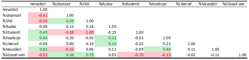
The internal structure of the party shares is even more striking. The correlation between %SNS and %Studenti is −1.00, which indicates an almost perfect mirror relationship across polling stations. This should not be overinterpreted as a sociological law. It is, above all, a compositional pattern: where the ruling list performs better, the student list performs worse, and vice versa. In a highly polarized local contest dominated by two effective poles, such a near-perfect negative relationship can emerge because the two vote shares absorb most of the competitive variation. This is analytically useful, but it also means that later interpretations must avoid treating the two shares as fully independent processes. They are structurally linked.
The smaller lists behave differently and deserve careful interpretation. The Russian Party has only a weak positive correlation with %SNS (r = 0.18) and a weak positive correlation with turnout (r = 0.13), which does not justify reading it as either a major anti-incumbent force or a clearly ruling-adjacent electoral satellite on statistical grounds alone. The Liberal list also shows only weak relationships with turnout (r = 0.00) and the ruling list (r = 0.19). The most interesting smaller list in the matrix is Koalicija 381, whose correlation with the ruling list is essentially zero (r = −0.03), but whose correlation with invalid ballots is positive (r = 0.40) and with the percentage of invalid ballots is even stronger (r = 0.46). That pattern is unusual but not self-explanatory. It may reflect geographically specific pockets of support, protest voting, or noise associated with small-sample local structures. It is not enough, by itself, to classify the list as either genuine opposition or quasi-opposition.
The matrix also suggests that turnout in Aranđelovac should not be read as a purely clean participation signal. Turnout is negatively correlated with the number of invalid ballots (r = −0.42) and with the percentage of invalid ballots (r = −0.33), while at the same time being positively correlated with the percentage voting outside the polling station (r = 0.38). This pattern already hints that what looks like “high turnout” may partly coincide with a more organized voting environment, one in which invalid ballots are fewer and out-of-polling-station voting is more common. Later sections show that both of these features are important for the ruling party’s performance.
The broader substantive conclusion is therefore stronger than a simple statement that “turnout helped SNS.” It is more precise to say that, in Aranđelovac, higher turnout was associated with a cluster of polling-station characteristics, fewer invalid ballots, more outside voting, and a higher ruling-party share, that together make turnout look politically asymmetric rather than neutral. That does not prove fraudulent turnout inflation. But it does mean that turnout cannot be treated as a benign contextual variable.
4.3 Limitations and caution
Correlation is a screening tool, not a final verdict. It does not identify causal direction, cannot distinguish between legal and illicit mechanisms, and is subject to ecological inference problems. It is also especially important here to interpret the −1.00 correlation between SNS and the student list as a feature of the local vote-share composition rather than as literal proof of one-to-one voter transfer. The smaller lists should also not be labelled “quasi-opposition” on the basis of correlation alone; such a claim would require campaign, organizational, and media evidence in addition to statistics.
4.4 Conclusion
Yes, the revised evidence supports the conclusion that higher turnout was more favorable to the ruling list than to the opposition. The core correlations are clear: turnout is positively associated with %SNS (r = 0.39) and negatively associated with %Studenti (r = −0.38), while the ruling and student lists themselves are nearly perfect opposites (r = −1.00). In forensic terms, this is a meaningful warning sign, especially because it aligns with the later regression and graphical findings.
5. Voting outside the polling station and vote shares
Did voting outside the polling station benefit the ruling candidate?
5.1 Intuitive logic
Voting outside the polling station exists to facilitate participation by voters who cannot physically come to vote. It is a legitimate institution, but it is also one of the least transparent parts of the electoral process. For that reason, election forensics treats it as a sensitive channel. The key question is whether this form of voting looks politically neutral or whether it is disproportionately associated with higher support for the ruling side.
5.2 Results and interpretation
The correlation matrix already points strongly in one direction. The percentage of voting outside the polling station (%Outside voting/%Glasali van) has a strong positive correlation with the ruling party’s vote share: r = 0.72. That is one of the strongest coefficients in the entire matrix. At the same time, the same variable has a strong negative correlation with the student list: r = −0.70. In practical terms, polling stations with more outside-the-polling-station voting tended also to be polling stations where SNS did substantially better and the main opposition did substantially worse. This is exactly the sort of asymmetry that requires closer explanation.
The regression results reinforce that reading. In Model 1, invalid ballots alone have a negative and highly significant association with the SNS share (−0.738). In Model 2, after turnout is added, the invalid-ballot coefficient remains negative and significant (−0.601), while turnout is positive but not statistically significant (0.433). In Model 3, however, once %Outside voting enters the model, it becomes strongly positive and highly significant (2.267), the model fit rises sharply to R² = 0.551, and the invalid-ballot coefficient shrinks to −0.200 and loses significance. This is a substantial structural change, not a cosmetic one. It suggests that outside voting captures a major part of the local pattern that simpler models were attributing, at least in part, to invalid-ballot variation.
Table 2: Regression analysis (dependent variable %SNS)
| Model 1 | Model 2 | Model 3 | |
| (Intercept) | 63.284*** | 30.624 | 34.742 |
| (2.672) | (22.406) | (18.095) | |
| Invalid | -0.738*** | -0.601** | -0.200 |
| (0.204) | (0.221) | (0.198) | |
| %Turnout | 0.433 | 0.196 | |
| (0.295) | (0.244) | ||
| %Outside voting | 2.267*** | ||
| (0.490) | |||
| Num.Obs. | 41 | 41 | 41 |
| R2 | 0.252 | 0.292 | 0.551 |
| R2 Adj. | 0.233 | 0.255 | 0.515 |
| p < 0.05, ** p < 0.01, *** p < 0.001 | |||
The correlation structure helps explain this shift. Outside voting is positively related to turnout (r = 0.38) and negatively related to the number of invalid ballots (r = −0.53). In other words, polling stations with more outside voting also tend to have higher turnout and fewer invalid ballots. This makes outside voting a strong candidate for a “carrier variable” that absorbs multiple dimensions of local electoral asymmetry. Once it is included in the regression, the residual independent role of invalid ballots becomes much smaller. That does not mean invalid ballots stop mattering. It means that part of their apparent effect may be riding through the same polling-station environment in which outside voting is more prevalent.
The urban–rural Welch test adds a territorial dimension to this interpretation. A Welch two-sample t-test showed that SNS support was significantly higher in rural areas than in urban areas, t(35.23) = 14.06, p<.0.01, 95% CI [16.53, 22.11]. The mean SNS share is 63.69% in rural polling stations and 44.37% in urban ones, with an extremely small p-value and a confidence interval that indicates a large substantive difference. This finding does not by itself establish wrongdoing in rural areas. Incumbents often perform better in rural settings for reasons that may be entirely political and social rather than fraudulent. But when the rural advantage is read together with the strong outside-voting effect, a plausible forensic interpretation is that the ruling side benefited most in precisely those settings where local dependence, weaker monitoring, or mobilization through less visible channels may have been easier.
Possible mechanisms include more effective mobilization of elderly or dependent voters, greater control over requests for home voting, pressure or informal influence in the execution of such voting, or weaker scrutiny of mobile ballot-box procedures. None of these channels can be proven from regression coefficients alone. But the combination of r = 0.72 in the correlation matrix and a 2.267 coefficient in Model 3 gives a strong empirical basis for the claim that outside-the-polling-station voting was not politically neutral in Aranđelovac.
5.3 Limitations and caution
Neither the correlation nor the regression can identify the precise mechanism. With only 41 polling stations, omitted variables remain possible, including age composition, settlement structure, and local organization. The evidence therefore does not justify a blunt statement that outside voting was manipulated. But it does justify a more careful and serious conclusion: this channel was statistically aligned with ruling-party advantage strongly enough to warrant suspicion and closer procedural scrutiny.
5.4 Conclusion
Yes, the evidence strongly supports the hypothesis that voting outside the polling station benefited the ruling candidate in Aranđelovac. The key numerical findings are the 0.72 correlation between %Outside voting and %SNS, the −0.70 correlation with the student list, and the 2.267 regression coefficient in Model 3. Taken together, these make outside voting one of the most important suspicious channels in the Aranđelovac result.
6. Invalid ballots and vote shares
Did invalid ballots benefit the ruling candidate?
6.1 Intuitive logic
In election forensics, invalid ballots are interesting because they sit at the boundary between voter intent, administrative judgment, and possible manipulation. A negative relationship between the winner’s vote share and invalid ballots may suggest that the winner performs better where fewer ballots are declared invalid. In theory, that can happen through at least two broad channels. One is the suppression of invalid ballots by converting questionable ballots into valid votes for the ruling side. The other is the selective production or concentration of invalid ballots in ways that reduce the competitive weight of other votes. Either way, invalid ballots become politically meaningful.
6.2 Results and interpretation
The correlation matrix helps sharpen this section considerably. The ruling-party share (%SNS) has a moderately strong negative correlation with the number of invalid ballots: r = −0.50. This means that polling stations with more invalid ballots tended to record a lower ruling-party percentage, while polling stations with fewer invalid ballots tended to record a higher ruling-party percentage. The student list shows the mirror image: %Studenti is positively correlated with the number of invalid ballots at r = 0.49. In other words, where invalid ballots are more numerous, the main opposition does relatively better; where invalid ballots are fewer, the ruling list does better. This is not proof of manipulation, but it is exactly the sort of asymmetry that makes invalid ballots forensically salient.
The matrix also shows that the percentage of invalid ballots behaves somewhat differently from the raw number. Its correlation with %SNS is only r = 0.06, essentially negligible, while its correlation with %Koalicija is r = 0.46 and with the number of invalid ballots it is r = 0.62. This distinction matters. It suggests that the raw count of invalid ballots carries more forensic signal vis-à-vis the ruling/opposition split than the invalid percentage does. One possible reason is that the raw number may be more sensitive to local administrative practice or polling-station scale, whereas the percentage mixes that information with other denominator effects. Either way, the main Mebane-style suspicion in Aranđelovac seems to attach more clearly to the number of invalid ballots than to their simple proportion.
The regression results are consistent with this reading, but they also add an important qualification. In Model 1, the coefficient on invalid ballots is −0.738; in Model 2 it remains −0.601 after turnout is added. These are not trivial coefficients, and the first two models therefore support the claim that fewer invalid ballots are associated with a higher SNS share. We ask that the numerical coefficient be interpreted substantively: if the winner’s share is measured relative to registered voters, then a reduction in invalid ballots is associated with an increase in the ruling candidate’s share on that broader base.
However, the multivariate picture becomes more complicated in Model 3. Once outside voting is introduced, the invalid-ballot coefficient falls to −0.200 and becomes statistically insignificant. That is a major interpretive point. It does not erase the suspicious invalid-ballot pattern. But it does suggest that invalid ballots are not acting as a fully autonomous mechanism. Instead, they appear to be part of a wider cluster of polling-station features in which outside voting is central. The matrix supports this interpretation, because the number of invalid ballots is itself negatively correlated with outside voting (r = −0.53). In effect, polling stations with more outside voting tend to have fewer invalid ballots and a higher ruling-party share. That is why the invalid-ballot effect weakens once outside voting is controlled.
Two theoretical readings remain possible. One is that fewer invalid ballots at ruling-leaning stations reflect tighter control over ballot validity, including the possible conversion of borderline ballots into valid votes for the ruling side. The other is broader: invalid ballots may simply be one visible trace of a local electoral environment in which the ruling side performs best under more organized, more controlled, and less transparent conditions. The data do not let us choose decisively between these two readings. But they clearly indicate that invalid ballots were not politically neutral in the Aranđelovac result.
6.3 Limitations and caution
Invalid-ballot analysis is inherently indirect. Neither correlations nor regressions can show how a particular ballot was handled or whether it was intentionally reclassified. Small sample size also matters. And because the invalid-ballot coefficient becomes insignificant once outside voting is added, one should resist the temptation to treat invalid ballots as the single dominant forensic channel in this election. They are better interpreted as one component of a larger suspicious structure.
6.4 Conclusion
Yes, the evidence supports the proposition that invalid ballots were linked to an outcome favorable to the ruling candidate. The key coefficients are r = −0.50 between invalid ballots and %SNS and r = 0.49 between invalid ballots and the student list, reinforced by the negative and significant invalid-ballot coefficients in Models 1 and 2. But the final interpretation must remain qualified: once outside voting is included, the invalid-ballot effect weakens sharply, which suggests that invalid ballots formed part of a broader asymmetrical electoral environment rather than a fully separate mechanism.
7. Turnout-based forensic regression in the Russian-school tradition
Does the turnout structure suggest that the ruling list benefited disproportionately from higher participation?
7.1 Intuitive logic
One of the better-known tools associated with the Russian school of election forensics examines the relationship between turnout and a candidate’s or list’s vote share measured not as a percentage of valid votes, but as a percentage of registered voters at each polling station. Formally, the model can be written as
$$\frac{V}{E} = \beta T + \alpha,$$
where \(T\) denotes turnout, \(V\) the number of votes won by the candidate or list, and \(E\) the number of registered voters at the polling station. The logic of the tool is straightforward. Under free and fair electoral conditions, one would expect the intercept \(\alpha\) to be approximately equal to the candidate’s baseline support, while the slope coefficient \(\beta\) should be close to zero. That would mean that higher turnout does not systematically translate into disproportionate gains for one political actor.
By contrast, if turnout is artificially inflated in ways that benefit one list, the coefficient \(\beta\) may become strongly positive, may approach 1, or may even exceed 1. In the most suspicious cases, a slope above 1 implies that every additional 100 voters who turn out are associated with more than 100 additional votes for the favored list. Under ordinary electoral arithmetic, that is impossible. It suggests that turnout growth is not simply bringing more voters into the process, but is mechanically linked to an implausibly large increase in support for one side. At the same time, the principal opponent may display a negative slope, indicating that as turnout rises, the opponent’s share among registered voters falls rather than rises.
7.2 Results and interpretation
In Aranđelovac, the graph provides a very clear result. For the ruling list Aleksandar Vučić – Aranđelovac, naša porodica!, the estimated regression is
$$y = -46.3 + 1.19T,$$
with adjusted \(R^2 = 0.46, F_{1,39} = 34.9, P < .001, n = 41\). For the opposition list Studenti za Aranđelovac, the estimated regression is
$$y = 43.7 – 0.192T,$$
with adjusted \(R^2 < 0.01, F_{1,39} = 0.843, P = .364, n = 41\).
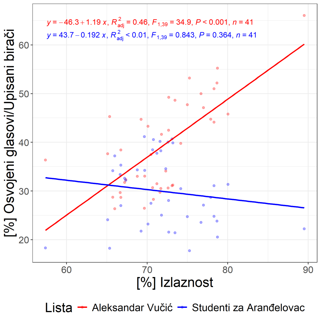
The ruling-list result is forensically striking. The estimated slope \(\beta = 1.19\) is not only positive and highly statistically significant, but also greater than 1. Interpreted literally, this means that an increase of 100 additional voters in turnout is associated with roughly 119 additional votes for the ruling list, measured against the base of registered voters. That is not a plausible electoral mechanism under ordinary competitive conditions. A slope larger than 1 implies that turnout growth is being converted into ruling-party gains at a rate that exceeds the number of newly participating voters themselves. This is exactly the kind of anomaly that made this tool famous in earlier election-forensics discussions, including the well-known Russian examples.
The opposition result points in the opposite direction, but much more weakly. The slope for the student-backed opposition list is negative, \(\beta = -0.192\), which means that as turnout rises, the opposition’s share among registered voters tends to decline slightly. This direction is consistent with the broader forensic suspicion that turnout benefited the ruling list more than the opposition. However, unlike the ruling-list coefficient, the opposition coefficient is not statistically significant. That means the graph does not justify a strong standalone claim that turnout systematically depressed opposition support in Aranđelovac. What it does show very clearly is that the ruling list had a highly unusual and highly significant positive turnout conversion pattern.
This result should be read together with the earlier sections of the Aranđelovac report. The ordinary turnout analysis already showed that higher turnout was associated with a better result for the ruling side and a worse result for the opposition. The current tool sharpens that conclusion by moving from simple correlation to a more demanding forensic interpretation. It shows not merely that turnout and ruling-party support moved together, but that the estimated conversion of turnout into ruling-party votes is implausibly steep. That makes this section one of the strongest pieces of evidence in the Aranđelovac case.
7.3 Limitations and caution
Even so, this method should not be treated as judicial proof on its own. A steep positive slope, even an unusually steep one, is still a statistical signal rather than direct evidence of a specific mechanism. In principle, one could imagine unusually strong mobilization of one side, spatial clustering of highly loyal voters, or other organizational processes that would generate a positive relationship. What makes the present case suspicious is not merely that the slope is positive, but that it is greater than 1, highly significant, and consistent with several other warning indicators discussed elsewhere in the report.
It is also important to remember that the opposition slope is negative but not significant. Therefore, the strongest conclusion from this graph is not that both sides behave in a perfectly symmetrical suspicious way, but that the ruling side shows an anomalously strong turnout-conversion pattern. That distinction matters for analytical precision. The graph is strongest as evidence of disproportionate benefit to the ruling list, not as equally strong evidence of direct suppression of the opposition.
Finally, this method uses vote share relative to registered voters, not relative to valid votes cast. That is exactly why the interpretation of \(\beta\) can become so powerful. But it also means the result must be explained carefully, so that readers understand why a slope greater than 1 is mathematically and politically problematic.
7.4 Conclusion
Yes, this turnout-based forensic regression strongly supports the hypothesis that the ruling list in Aranđelovac benefited disproportionately from higher turnout. The key reason is the estimated slope of \(\beta = 1.19\) for the ruling list, which is not only highly statistically significant but also greater than 1. That is a highly anomalous result and one of the strongest warning signs in the Aranđelovac analysis. By contrast, the opposition slope is negative but not statistically significant, so the main forensic weight of this section falls on the implausibly steep and significant turnout effect for the ruling side.
8. Graphical analysis of vote shares by turnout
We state that, among the five recent elections shown in the Aranđelovac turnout plots, the ruling side’s slope was negative but statistically insignificant in the 2017 presidential and 2023 parliamentary elections, while in the remaining elections, including the 2026 local election, it was positive and statistically significant. We further state that the 2026 local election shows the strongest and most highly significant positive relationship between turnout and the ruling party’s vote share. The corresponding opposition plot shows the mirror pattern: where the slope becomes positive in earlier elections it is not significant, but in the 2026 local election the slope is strongly negative and highly significant. We also emphasize a particularly striking symmetry: at the local election, a 1% increase in turnout corresponds to roughly +0.77 percentage points for the ruling side and −0.77 percentage points for the opposition.
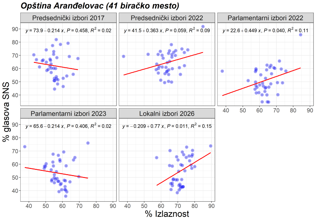
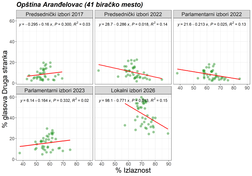
This is one of the strongest pieces of evidence in the Aranđelovac file. It suggests not only that turnout benefited the ruling side in 2026, but that the local-election pattern is sharper than in at least part of the recent electoral history. In forensic terms, a consistently positive ruling slope combined with a consistently negative opposition slope is exactly the kind of recurring structure that raises concern about asymmetric mobilization or turnout-related electoral distortion.
9. Klimek curves
With only 41 polling stations, the cumulative curves are informative but not decisive. The ruling and opposition curves almost coincide up to about 73% turnout; between roughly 73% and 78%, the opposition curve lies above the ruling one; after about 78% turnout, the ruling curve begins to rise faster than the opposition curve. This does not produce a clean, dramatic “non-democratic” signature of the kind shown in the original Klimek examples, and the small number of observations, especially at the high-turnout end, makes strong inference difficult.
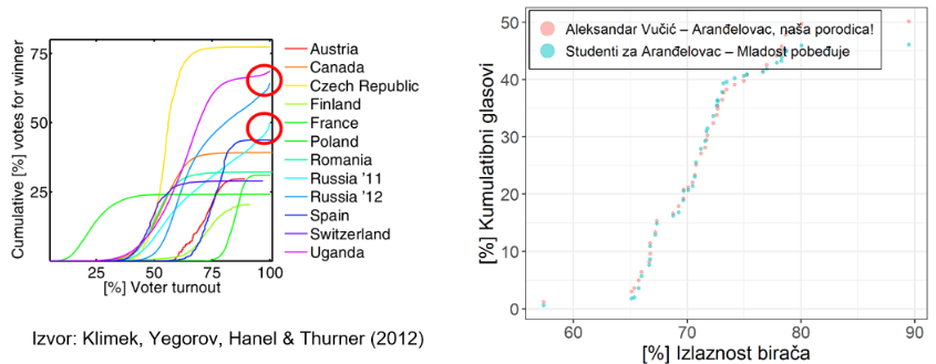
The appropriate conclusion is therefore limited: the Klimek analysis does not independently establish manipulation in Aranđelovac, but neither does it neutralize the more substantial warning signs emerging from turnout asymmetry, outside voting, and the finite-mixture results.
10. Election fingerprints
We place more weight on the election fingerprints than on the Klimek curves. We explicitly state that the local-election marginal distribution shows two peaks, which permits suspicion, and that the heat map indicates two clusters at approximately the same turnout level, one of which is associated with a much higher ruling-party vote share. We also draw attention to a smudge elongated toward high winner percentages and ask whether the fingerprint structure changed across the last five elections. This is important because a two-cluster or elongated fingerprint can be compatible with deep heterogeneity in local voting environments, but it can also be compatible with a layered electoral field in which one subset of polling stations behaves under more controlled or less competitive conditions.
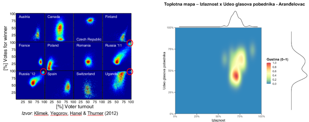
With only 41 observations, the method again requires caution. But when interpreted together with the turnout and outside-voting evidence, the fingerprint structure does not look electorally innocent.
11. Finite-mixture model
The finite-mixture results remain among the strongest warning signs in the Aranđelovac file. The analysis classifies the 41 polling stations into three groups: 18 “no fraud” stations, 9 “incremental fraud” stations, and 14 “extreme fraud” stations. The mean turnout and mean winner share increase systematically across those classes: about 69.7% turnout / 43.7% winner share in the no-fraud class, 73.0% / 56.6% in the incremental-fraud class, and 74.1% / 66.3% in the extreme-fraud class. The report further attributes about 44.6% of the winner’s total votes to the fraud-type classes taken together.
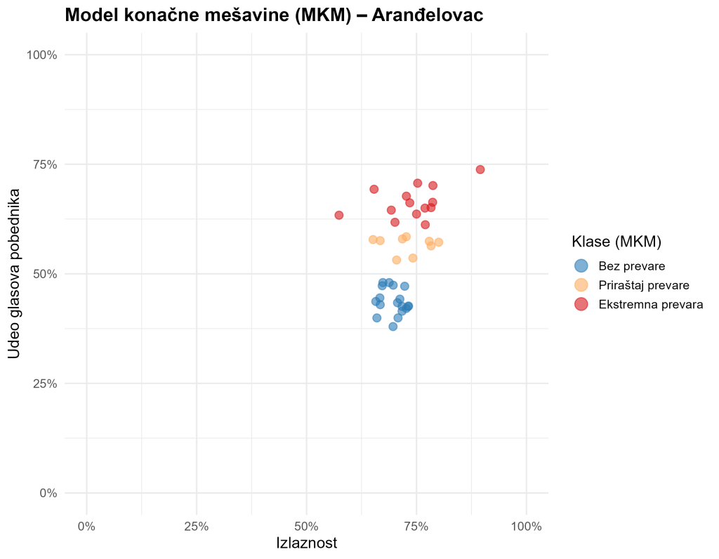
This is a serious forensic warning signal, but it is also the method that requires the most caution in a small municipality. Finite-mixture estimates are sensitive to specification, cluster separation, and sample size. At 41 polling stations, the result is analytically striking but should still be presented as strongly suggestive rather than mechanically conclusive. Even so, the existence of a sizable extreme-fraud class is difficult to dismiss when it aligns with the turnout, outside-voting, and fingerprint evidence.
12. Executive Summary
Data and preparation
This report analyzes polling-station-level data for the 2026 local election in Aranđelovac using a multi-method election-forensics framework. The analysis combines a correlation matrix, regression models, turnout graphics, an urban–rural comparison, Klimek curves, election fingerprints, and a finite-mixture model. Because the municipality contains only 41 polling stations, each method must be interpreted cautiously; however, the cumulative convergence of several methods remains highly informative.
Turnout and vote shares
Higher turnout appears to have benefited the ruling list more than the opposition. The correlation matrix shows r = 0.39 between turnout and %SNS, and r = −0.38 between turnout and the student list. The ruling and student shares are themselves almost perfect opposites (r = −1.00), which confirms a highly polarized local electoral structure.
Voting outside the polling station and vote shares
This is one of the strongest suspicious channels in the Aranđelovac result. The correlation between outside voting and the ruling-party share is 0.72, while the correlation with the student list is −0.70. In the multivariate regression, outside voting becomes strongly positive and highly significant (2.267), while model fit rises sharply.
Invalid ballots and vote shares
Invalid ballots initially behave in a Mebane-consistent way. Their number is negatively correlated with the ruling-party share (r = −0.50) and positively correlated with the student list (r = 0.49). However, once outside voting is included in the regression, the invalid-ballot coefficient weakens and loses significance, which suggests that invalid ballots are part of a wider suspicious pattern rather than an isolated mechanism.
Turnout-based forensic regression in the Russian-school tradition
In the additional check based on the Russian school of election forensics, Aranđelovac displays one of the most striking warning signs in the entire analysis. The estimated slope coefficient for the ruling list is \(\beta = 1.19\) and is highly statistically significant, meaning that higher turnout was associated with an implausibly large increase in votes for the ruling side relative to the number of registered voters. Such a result is difficult to reconcile with the normal pattern of free and fair elections, because it suggests that the ruling list was gaining more votes from additional turnout than would be mathematically possible under regular conditions. The opposition list did show a negative slope, but without statistical significance, so the main conclusion of this tool remains clear: in Aranđelovac, turnout functioned as a strongly asymmetric channel that disproportionately benefited the ruling side.
Graphical analysis by turnout
The 2026 local election stands out from several earlier elections. The ruling side benefits more from higher turnout, while the opposition loses more as turnout rises. According to the analysis, the latest local election shows the strongest positive ruling slope and the strongest negative opposition slope among the five elections plotted.
Klimek curves
The Klimek analysis is inconclusive in the strict sense because the number of polling stations is small. The cumulative curves do not provide a dramatic standalone signature of manipulation, but neither do they contradict the more substantial concerns raised by the other methods.
Election fingerprints
The fingerprint analysis is suspicious. The local-election marginal distribution appears bimodal, and the heat map suggests two clusters at similar turnout levels but markedly different winner-share levels. This is not decisive on its own, but it is difficult to regard as ordinary once read together with the other findings.
Finite-mixture model
The finite-mixture model produces one of the strongest warnings in the entire file. A substantial number of polling stations are classified into incremental- and extreme-fraud clusters, and the total estimated fraud-share component is about 44.6%. This must be interpreted cautiously because of the small sample size, but it is still analytically serious.
Overall assessment
Taken together, the Aranđelovac findings provide meaningful grounds for suspicion that the election was not conducted under conditions of fully fair and neutral competition. No single method proves manipulation by itself. But the cumulative structure, turnout asymmetry, a very strong outside-voting effect, a suspicious invalid-ballot relationship, unusual fingerprints, and a strongly suggestive finite-mixture output, supports the view that the result is consistent with a distorted and potentially manipulated electoral environment. These findings should be interpreted in light of the broader pre-election conditions discussed in earlier blog posts, including unequal media treatment and broader asymmetries of political power.
13. Methodological appendix
This report uses seven complementary election-forensics approaches. Correlation analysis serves as an initial screening device for systematic polling-station-level relationships. Regression analysis tests whether those relationships remain when multiple explanatory variables are considered jointly. Turnout graphics evaluate whether higher participation disproportionately helps the ruling side and harms the opposition. Klimek curves examine whether cumulative vote growth behaves more like a democratic plateau or a suspicious acceleration pattern. Election fingerprints inspect the joint distribution of turnout and winner share, together with the shape of their marginal distributions. The urban–rural comparison tests whether the ruling side’s support is territorially concentrated in a way that may matter for interpretation. Finally, the finite-mixture model classifies polling stations into latent regular and suspicious types and estimates the winner’s vote share associated with each class. None of these methods is conclusive on its own, especially with only 41 observations. But together they provide a structured framework for assessing electoral integrity.
Director of Wellington based My Statistical Consultant Ltd company. Retired Associate Professor in Statistics.
Has a PhD in Statistics and over 45 years experience as a university professor, consultant, international researcher and government advisor.