Reading Time: 6 minutes

Series: “Election Forecasting: Between Statistics, Politics, and Uncertainty” — Election Forensics

After an election, a second competition usually begins. Parties are no longer the only contestants. Pollsters, media outlets, commentators, and their critics start calculating who “got it right”, who “missed”, who came closest, and who, inevitably, must have been lying.

A calculator is useful. But before distributing medals or accusations according to absolute percentage-point error, we need to ask a boring but decisive question: Was the number we are comparing with the election result actually an election forecast?

A survey conducted in June measures responses collected in June. An election held in late October records votes cast by people who actually turned out in late October. Between those two moments there can be an entire campaign, changes in electoral lists, new political events, mobilisation, demobilisation, and genuine changes of mind.

One of the central messages of this series is therefore simple: a public-opinion poll is not automatically an election forecast.

The same poll can lead to different election results

Chapter 2 uses an intentionally simple example. Imagine two political settings with exactly the same observed poll: List A at 42%, List B at 36%, and others at 22%.

If supporters of all groups turn out at broadly similar rates, the final vote remains relatively close to the survey relationship. But if List A’s supporters are mobilised much more effectively while List B’s supporters are more likely to stay home, exactly the same poll can generate a substantially different election result.

This is not exotic statistics. It is simply the reminder that only people who actually vote can cast ballots. Chapter 2 therefore separates political preference from political participation and stresses that parties with identical survey support can obtain different results if their supporters have different turnout propensities.

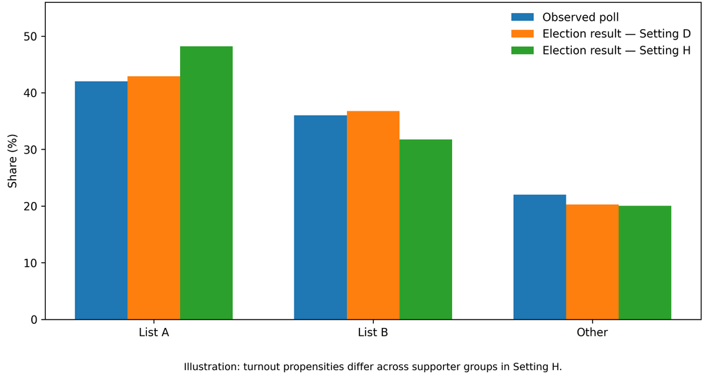
[Figure 2.3. Same poll, different turnout, different result]

“I will definitely vote” is not the same as voting

Turnout questions illustrate the problem perfectly. NSPM’s latest survey reports that 79.8% of respondents say they will “definitely” vote and another 13.3% say they will probably vote. Faktor Plus’s September survey, as reported publicly, put turnout at 62%, with 22% saying they would not vote and 16% saying they did not know.

Does that prove that one pollster must be wrong? No.

The questions may have been formulated differently. Survey modes may generate different levels of socially desirable responses. One number may be a raw self-reported intention while another is a more restrictive estimate. The political environment may also have changed between the fieldwork periods.

This is exactly why methodology matters. Without it, we compare two percentages as if they came from identical thermometers when one may be measuring air temperature and the other how warm respondents feel.

Mobilisation is not preference

Political commentary often treats survey support as a reservoir of votes: if a party is at 40%, it somehow “owns” that 40%. But polls do not own voters.

A person can have a clear political preference and still abstain. Another can remain weakly engaged until a campaign, local organisation, political event, or sense of threat mobilises them.

Hybrid political environments may contain additional mechanisms: clientelist networks, workplace or institutional dependence, different forms of pressure, and unusually intensive organisational mobilisation. But here again we are not entitled to pre-select the direction of the effect. The literature discussed in Chapter 2 shows precisely why competition, coercion, and clientelism do not generate one universal turnout pattern.

If you believe that public-sector employment, a clientelist network, or student mobilisation changes turnout, that is a legitimate hypothesis.

The next questions are: by how much, for whom, where, and does the relationship repeat? Without those answers, we do not have a forecast correction. We have a scenario.

A public-sector job is not a ballot paper

In Serbian political debate, public-sector employment is sometimes treated almost like a party membership card. Politically, one can understand why. Statistically, it is far too crude.

Chapter 2 explicitly rejects coding a public-sector employee automatically as a government voter. The relevant question is whether employment status predicts turnout or vote choice after age, education, region, and other characteristics are taken into account — and, critically, whether including that variable improves predictions for elections not used to estimate the relationship.

That sounds less impressive on television than saying “we know how the public enterprises vote”. It has one advantage: it can be tested.

Exactly the same discipline should apply to young voters. The political visibility of university students does not automatically tell us how many young citizens will turn out or that every young voter supports the Student List. Youth mobilisation may be electorally important, but its scale needs to be measured rather than assumed.

Who “won” the polling competition?

After election day, a special form of retrospective science often emerges. Take the final result, calculate the distance from each pre-election poll, and declare the closest pollster methodologically superior. That can be useful only if we first ask what the surveys were actually measuring.

CRTA’s June fieldwork is not a forecast of a late-October election merely because it asked respondents how they would vote. It is first and foremost a measurement of reported preferences in June. Faktor Plus’s second-half-of-September poll is much closer to election day. NSPM’s fieldwork from 25 September to 5 October is closer still, but its data-collection mode differs.

If the election result turns out to be closer to one of them, that is useful information. But it does not automatically mean that the others were “fake”. Evaluating a polling organisation requires repeated elections, fieldwork dates, survey mode, treatment of undecided voters, and systematic errors by party. One accurate hit can reflect skill. It can also reflect luck.

“But they differ by ten points!”

That is a legitimate objection. When CRTA in June reports a Student List advantage while Faktor Plus in September reports a double-digit advantage for the governing list, the disagreement is large enough to demand serious investigation.

Serious investigation, however, is not the same as appointing one poll as the truth. In commentaries labelling CRTA or NSPM surveys “fake”, Faktor Plus is often treated as the known “real and correct” value, and divergence from it is then used as proof of falsification. That is circular reasoning. First declare one poll true, then use it to prove that the others are false.

It would be equally poor methodology to treat CRTA as the reference truth and dismiss every poll more favourable to the government as regime propaganda.

The scientific answer is less satisfying. We need more evidence.

What belongs in the forecast model?

This is where Chapter 2 introduces one of the distinctions I consider most important in the book.

Some effects can be estimated reasonably well. If we have enough historical surveys from a pollster, we can investigate whether it systematically over- or underestimates support for particular parties. Such a house effect may enter the central forecast together with uncertainty about its size.

Other effects are only partially identified. We may have evidence that turnout in a particular group is likely to be higher than before but not enough evidence to specify exactly how much. That belongs in sensitivity analysis.

And some mechanisms may be politically plausible while their magnitude remains essentially unknown. “Hidden opposition voters” without validation data are a good example. They should not silently become two or three extra opposition points in the main forecast. Their proper place is an explicitly labelled scenario.

The rule should apply regardless of which political side would benefit from the adjustment.

Election forensics is not a statistical eraser

Historical election results are commonly used as inputs to future forecasting models. What should we do when there are serious reasons to question the quality of some historical observations? One extreme is to treat every official number as equally reliable and ignore all concerns. The opposite extreme is to “correct” or remove results whenever a statistical pattern looks suspicious. Neither is satisfactory.

Chapter 2 recommends a robustness approach: use official historical data as the baseline, but test how much the forecast changes under pre-specified alternative treatments of observations that deserve scrutiny. A statistical anomaly then becomes a reason for sensitivity analysis, not permission for the analyst to recount the election on a laptop. That is an important boundary between election forecasting and election forensics.

Pollsters are also educators

All of this returns us to the educational responsibility of polling organisations.

If the public sees only “List A 45%, List B 42%”, many people will interpret those numbers almost like a currency exchange rate. If the same release explains that the 45% refers to decided voters, that 18% of the sample remains undeclared, that fieldwork ended two weeks earlier, and that the survey measures current stated intention rather than a guaranteed election result, the audience receives a fundamentally different message.

That does not weaken the poll. It makes it more serious.

Media outlets have the same responsibility. “A leads by three points” may attract more clicks than “A leads by three points among declared respondents in a telephone survey whose fieldwork ended two weeks ago”. But the second statement is closer to what is actually known.

In a highly polarised society, this is not pedantry. Incomplete presentation can create unjustified confidence before the election and, after the election, make every polling error look like evidence of fraud or fabrication.

Pouring petrol on a political fire does not become harmless because the bottle is labelled “public opinion research”.

The most important question: what is the mechanism?

When a poll and an election result differ, many explanations are possible. Public opinion changed. Undecided voters made up their minds. Sampling was biased. One side mobilised more effectively. Some respondents concealed preferences. A likely-voter model failed. Electoral coalitions changed.

Perhaps the research really was poor. But before selecting the explanation, we need to identify the mechanism.

That is the central message of Chapter 2 and perhaps the best protection against partisan interpretation of polling: first the mechanism, then the evidence, and only then the correction. Not the other way around.